The Tafel plot shown below is the most ideal polarization curve that can be constructed. It was built using data points computed by the Butler-Volmer equation with the following parameters: T = 298 K, n꜀ = nₐ = 2, α = 0.5, i₀ = 10⁻¹¹ A. Any real polarization curve is “worse” from the point of view of Tafel analysis.
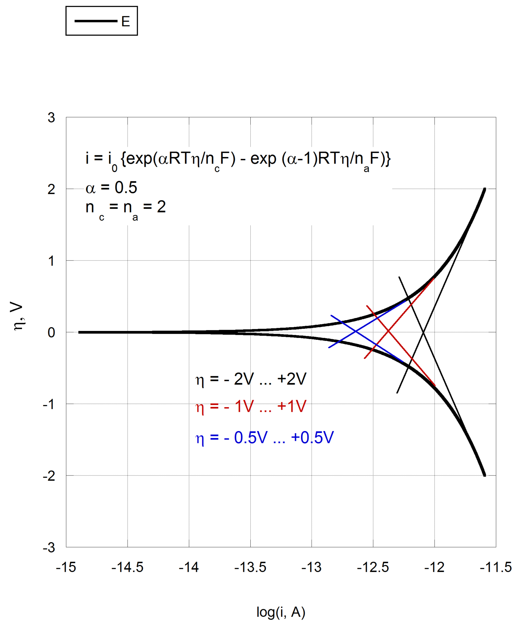 Three sets of Tafel slopes were fitted to this plot. The black slopes cover an overvoltage range of ±2.0 V, the red slopes cover ±1.0 V, and the blue slopes cover ±0.5 V. As seen in the figure, while the corrosion potentials obtained from all three fits are identical (and equal to the true corrosion potential), the corrosion currents depend very strongly on the chosen overpotential range: the current extracted from the largest range is five times higher than that from the smallest.
The reason is fundamental, not computational. A truly linear region on a Tafel plot exists only at sufficiently large overpotentials, where the back-reaction is negligible. At small overpotentials — close to E꜀ₒᵣᵣ — both anodic and cathodic partial currents are comparable, the curve is inherently non-linear, and any straight line fitted through it is an approximation at best. The problem is that for almost any potential range one can find a visually convincing linear segment. These segments differ, however, and the larger the range, the larger the apparent Tafel slopes and the extracted corrosion current.
In practice, polarization curves can usually only be measured over a range of ±0.25 V, sometimes less. Real curves are further distorted by additional processes and noise. Two examples measured for the corrosion of a magnesium alloy in salt water are shown below.
Three sets of Tafel slopes were fitted to this plot. The black slopes cover an overvoltage range of ±2.0 V, the red slopes cover ±1.0 V, and the blue slopes cover ±0.5 V. As seen in the figure, while the corrosion potentials obtained from all three fits are identical (and equal to the true corrosion potential), the corrosion currents depend very strongly on the chosen overpotential range: the current extracted from the largest range is five times higher than that from the smallest.
The reason is fundamental, not computational. A truly linear region on a Tafel plot exists only at sufficiently large overpotentials, where the back-reaction is negligible. At small overpotentials — close to E꜀ₒᵣᵣ — both anodic and cathodic partial currents are comparable, the curve is inherently non-linear, and any straight line fitted through it is an approximation at best. The problem is that for almost any potential range one can find a visually convincing linear segment. These segments differ, however, and the larger the range, the larger the apparent Tafel slopes and the extracted corrosion current.
In practice, polarization curves can usually only be measured over a range of ±0.25 V, sometimes less. Real curves are further distorted by additional processes and noise. Two examples measured for the corrosion of a magnesium alloy in salt water are shown below.
.PNG)
The solid-line curve is acceptable (though somewhat noisy in the anodic branch), and the Tafel slopes should be fitted over the maximum available range (red lines). The dashed-line curve is not only noisier — its cathodic branch shows a clear deviation at higher currents, indicative of an additional process. For magnesium in salt water this is most likely the anomalous hydrogen evolution accompanying active dissolution (the so-called negative difference effect), or the onset of pitting. Whatever the cause, this region must be excluded, and the cathodic fit limited to where the curve still follows Tafel behavior (blue lines). Practical rules for building Tafel slopes: 1. Use the largest available potential range that is free from additional processes. 2. Be prepared to encounter polarization curves for which a correct Tafel analysis is simply impossible. 3. Always cross-check the results by independent methods — for example, EIS or linear polarization resistance (Stern–Geary).